Cosmic Microwave Background

The Cosmic Microwave Background (CMB) radiation is a very faint but observable form of radiation that is coming to us (and to other places too) from all directions. (By ‘radiation’ here is meant photons of light, or electromagnetic waves, from a wide range of possible frequencies or energies.) In today’s standard model of cosmology, this radiation is believed to emanate from about a time 200,000 to 400,000 years after the Big Bang – a timeframe known as ‘last scattering’ because that was when superheavy collisions between photons of light and other particles (electrons, protons, neutrons, etc) eased off to a degree that photons can ‘escape’ into the expanding space. At the time of last scattering, this radiation was very hot, around K (in the Kelvin scale). And in time, as space expanded, radiation cooled to its currently observed value of K.

One of the amazing facts about this radiation is that it almost perfectly matches Planck’s radiation formula (discovered in 1900) for a black body:

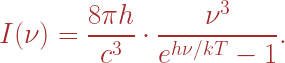
In this formula, is the frequency variable (a positive real number that gives the number of cycles per second of a wave) and is the energy density as a function of frequency .

The other variables are: is the temperature of the black body which is assumed to be in equilibrium (so the temperature is uniformly constant throughout the body of radiation), is the speed of light in vacuum, is Planck’s constant, and is Boltzmann’s constant from statistical mechanics.

If you plot the graph of this energy density function (against ) you get a curve that looks like a skewed ‘normal distribution’. Here are some examples I hijacked from the internet:

Various Planck radiation density graphs depending on temperature T.

Here you see various plots of Planck’s function for different temperatures . The horizontal axis labels the frequency , and the vertical gives the energy density per frequency. (Please ignore the rising black dotted curve.)

You’ll notice that the graphs have a maximum peak point. And that the lower the temperature, the smaller the frequency where the maximum occurs. Well, that’s what happened as the CMB radiation cooled from a long time ago till today: as the temperature T cooled (decreased) so did the frequency where the peak occurs.

To those of us who know calculus, we can actually compute what frequency gives maximum density and give our answer in terms of the temperature . All we do is compute the derivative of with respect to and set it to zero and solve the resulting equation for . You will get an equation whose solution isn’t so trivial to solve, so we’ll need some software or a calculator to approximate it. Anyway, I worked it out (and you can check my answer) and obtained the following:

(The equal sign here is an approximation!)

The is the frequency that gives maximum density and as you can see it is a straight linear function of temperature. The greater the temperature, the proportionately greater the max frequency. The colder the temperature gets the smaller the max-frequency gets, and from Planck’s energy equation , so also does the energy of the radiation drop.

Now plug in the observed value for the temperature of the background radiation, which is (degrees Kelvin), and working it out we get (approximately)

This frequency lies inside the microwave band which is why we call it the microwave radiation! (Even though it does also radiate in other higher and lower frequencies too but at much less intensity!)

Far back in time, when photons were released from their collision `trap’ (and the temperature of the radiation was much hotter) this max frequency was not in the microwave band.

Homework Question: what was the max-frequency at the time of last scattering? What frequency band does it belong to? In the visible range? Infrared? Ultraviolet? Higher still? (I’m dying to know! 😉 )

(It isn’t hard as it can be figured from the data above.)

Anyway, I thought working these out was fun.

The CMB radiation was first discovered by Penzias and Wilson in 1965. According to their measurements and calculations (and polite disposal of the pigeons nesting in their antenna!), they measured the temperature as being K plus or minus 1 Kelvin. (So the actual value that was confirmed later, namely 2.726, fits within their range.) The frequency of radiation that they detected, however, was not the maximum yielding one but was (as they had it in the title of their paper) 1080 Mc/s — which is ‘mega cycles per second’ and is the same as MHz (megahertz). The wavelength value corresponding to this is 7.35 cm. To do the conversion between wavelength and frequency for electromagnetic waves we use the simple formula

where c is the speed of light (in vacuum).

And that’s the end of our little story for today!

Cheers, Sam Postscript.

The sacred physical constants:

Planck’s constant

Boltzmann’s constant

Speed of light .  

Richard Feynman on Erwin Schrödinger

I thought it is interesting to see what the great Nobel Laureate physicist Richard Feynman said about Erwin Schrödinger’s attempts to discover the famous Schrödinger equation in quantum mechanics (see quote below). It has been my experience in reading physics that this sort of “heuristic” reasoning is part of doing physics. It is a very creative (sometimes not logical!) art with mathematics in attempting to understand the physical world. Dirac did it too when he obtained his Dirac equation for the electron by pretending he could take the square root of the Klein-Gordon operator (which is second order in time). Creativity is a very big part of physics.

 

“When Schrödinger first wrote it down [his equation],

he gave a kind of derivation based on some heuristic

arguments and some brilliant intuitive guesses. Some

of the arguments he used were even false, but that does

not matter; the only important thing is that the ultimate

equation gives a correct description of nature.”

                                    — Richard P. Feynman

(Source: The Feynman Lectures on Physics, Vol. III, Chapter 16, 1965.)

 

 

 

Principles of quantum theory

One beautiful summer morning I spent a couple hours in a park reflecting on what I know about quantum mechanics and thought to sketch it out from memory. (A good brain exercise to recapture things you learned and admire.) This note is an edited summary of my handwritten draft (without too much math).

Being a big subject, I will stick to some basic ideas (or principles) of quantum theory that may be worth noting.

Two key concepts are that of a `state’ and that of an ‘observable’.

The former describes the state of the system under study. The observable is a thing we measure. So for example, an electron can be in the ground state of an atom – which means that it is in `orbital’ of lowest energy. Then we have other states that it can be in at higher energies.

The observable is a quantity distinct from a state and one that we measure. Such as for example measuring a particle’s energy, its mass, position, momentum, velocity, charge, spin, angular momentum, etc.

QM gives us principles / interpretations by how states and observables can be mathematically described and how they relate to one another. So here is the first principle.

Principle 1. The state of a system is described by a function (or vector) ψ. The probability density associated with it is given by |ψ|².

This vector is usually a mathematical function of space, time (sometime momentum) variables.

For example, f(x) = exp(-x^2) is one such example. You can also have wave examples such as g(x) = exp(-x^2) sin(x) which looks like a localized wave (a packet) that captures both being a particle (localized) and a wave (due to the wave nature of sin(x)). This wave nature of the function allows it to interfere constructively or destructively with other similar functions — so you can have interference! In actual QM these wavefunctions involve more variables that one x variable, but I used one variable to illustrate.

Principle 2. Each measurable quantity (called an ‘observable’) in an experiment is represented by a matrix A. (A Hermitian matrix or operator.)

For example, energy is represented by the Hamiltonian matrix H, which gives the energy of a system under study. The system could be the hydrogen atom. In many or most situations, the Hamiltonian is the sum of the kinetic energy plus the potential energy (H = K.E. + V).

For simplicity, I will treat a measurable quantity and its associated matrix on equal footing.

From matrix algebra, a matrix is a rectangular array of numbers – like, say, a square array of 3 by 3 numbers, like this one I grabbed from the net:

Turns out you can multiply such things and do some algebra with them.

Two basic facts about these matrices is:

(1) they generally do not have the commutative property (so AB and BA aren’t always equal), unlike real or complex numbers,

(2) each matrix A comes with `magic’ numbers associated to it called eigenvalues of A.

For example the matrix

(called diagonal because it has all zeros above and below the diagonal) has eigenvalues 1, 4, -3. (When a matrix is not diagonal we have a procedure for finding them. Study Matrix or Linear Algebra!)

Principle 3. The possible measurements of a quantity will be its eigenvalues.

For example, the possible energy levels of an electron in the hydrogen atom are eigenvalues of the associated Hamiltonian matrix!

Principle 4. When you measure a quantity A when the system is in the state ψ the system `collapses’ into an eigenstate f of the matrix A.

Therefore the system makes a transition from state ψ to state f (when A is measured).

So mathematically we write

Af = af

which means that f is an eignstate (or eigenvector) of A with eigenvalue a.

So if A represents energy then `a’ would be energy measurement when the system is in state f.

For a general state ψ we cannot say that Aψ = aψ. This eigenvalue equation is only true for eigenstates, not general states.

Principle 5. Each state ψ of the system can be expressed as a superposition sum of the eigenstates of the measurable quantity (or matrix) A.

So if f, g, h, … are the eigenstates of A, then any other state ψ of the system can be expressed as a superposition (or linear combination) of them:

ψ = bf + cg + dh + …

where b, c, d, … are (complex) numbers. Further, |c|^2 = probability ψ will `collapse’ into the eigenstate g when measurement of A is performed.

These principles illustrate the indeterministic nature of quantum theory, because when measurement of A is made, the system can collapse into any one of its many eigenstates (of the matrix A) with various probabilities. So even if you had the ‘exact same’ setup initially there is no guarantee that you would see your system state change into the same state each time. That’s non-causality! (Quite unlike Newtonian mechanics.)

Principle 6. (Follow-up to Principles 4 and 5.) When measurement of A in the state ψ is performed, the probability that the system will collapse into the eigenstate vector φ is the dot product of Aψ and φ.

The latter dot product is usually written using the Dirac notation as <φ|A|ψ>.  In the notation above, this would be same as |c|^2.

Next to the basic eigenvalues of A, there’s also it’s `average’ value or expectation value in a given state. That’s like taking the weighted average of tests in a class – with weights assigned to each eigenstate based on the superposition (as in the weights b, c, d, … in the above superposition for ψ). So we have:

Principle 7. The expected or average value of quantity A in the state described by ψ is <ψ|A|ψ>.

In our notation above where ψ = bf + cg + dh + …, this expected value is

<ψ|A|ψ> = |b|^2 times (eigenvalue of f)  + |c|^2 times (eigenvalue of g) + …

which you can see it being the weighed average of the possible outcomes of A, namely from the eigenvalues, each being weighted according to its corresponding probabilities |b|^2, |c|^2, … .

In other words if you carry out measurements of A many many times and calculate the average of the values you get, you get this value.

Principle 8. There are some key complementary measurement observables. (Classic example: Heisenberg relation QP – PQ = ih.)

This means that if you have two quantities P and Q that you could measure, if you measure P first and then Q, you will not get the same result as when you do Q first and then P. (In Newton’s mechanics, you could at least in theory measure P and Q simultaneously to any precision in any order.)

Example, position and momentum are complementary in this respect — which is what leads to the Heisenberg Uncertainty Principle, that you cannot measure both the position and momentum of a subatomic particle with arbitrary precision. I.e., there will be an inherent uncertainty in the measurements. Trying to be very accurate with one means you lose accuracy with they other all the more.

From Principle 8 you can show that if you have an eigenstate of the position observable Q, it will not be an eigenstate for P but will be a superposition for P.

So `collapsed’ states could still be superpositions! (Specifically, a collapsed state for Q will be a superposition, uncollapsed, state for P.)

That’s enough for now. There are of course other principles (and some of the above are interlinked), like the Schrodinger equation or the Dirac equation, which tell us what law the state ψ must obey, but I shall leave them out. The above should give an idea of the fundamental principles on which the theory is based.

Have fun,
Samuel Prime