Largest Triangle inside a Curvilinear Triangle

In the diagram shown we have part of a circle of radius whose center is at the point and which is tangent to the x and y axes — though the graph is drawn for R = 2, we want to work with general R.

Our focus is on the region under the circle above the x-axis. The question is: what is the maximum area that a triangle inside this region can have?

It may occur to you that there is a reasonable `quick’ answer, but the point of the problem is to reason it out carefully so you more or less have a proof that you do indeed get a maximum area. Since the region is concave, the vertices of a triangle cannot be so that one is too close to the far right while another vertex close to the far top left (or else the triangle would not be fully inside the region).

Have fun!

Two Little Circles

In the diagram shown we see a big circle of radius R that is tangent to both the x and y axes. What is the radius of the little circle to its southwestern corner? Express its radius in terms of R. (The little circle is also required to be tangent to the axes. The diagram is draw for a circle of radius 2 but we’re working with a general radius R.)

After having solved this problem, the next question will be this:

You can easily see that we can repeat the process by looking at the southwestern circles for ever and ever because there will always be a gap, and you get smaller and smaller circles with small radii. What if you add up all their radii? Do they add up? If so to what number do they add up, in terms of the original radius R. If they don’t add up, why don’t they?

Cosmic Microwave Background

The Cosmic Microwave Background (CMB) radiation is a very faint but observable form of radiation that is coming to us (and to other places too) from all directions. (By ‘radiation’ here is meant photons of light, or electromagnetic waves, from a wide range of possible frequencies or energies.) In today’s standard model of cosmology, this radiation is believed to emanate from about a time 200,000 to 400,000 years after the Big Bang – a timeframe known as ‘last scattering’ because that was when superheavy collisions between photons of light and other particles (electrons, protons, neutrons, etc) eased off to a degree that photons can ‘escape’ into the expanding space. At the time of last scattering, this radiation was very hot, around K (in the Kelvin scale). And in time, as space expanded, radiation cooled to its currently observed value of K.

One of the amazing facts about this radiation is that it almost perfectly matches Planck’s radiation formula (discovered in 1900) for a black body:

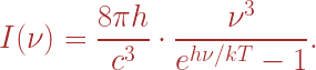
In this formula, is the frequency variable (a positive real number that gives the number of cycles per second of a wave) and is the energy density as a function of frequency .

The other variables are: is the temperature of the black body which is assumed to be in equilibrium (so the temperature is uniformly constant throughout the body of radiation), is the speed of light in vacuum, is Planck’s constant, and is Boltzmann’s constant from statistical mechanics.

If you plot the graph of this energy density function (against ) you get a curve that looks like a skewed ‘normal distribution’. Here are some examples I hijacked from the internet:

Various Planck radiation density graphs depending on temperature T.

Here you see various plots of Planck’s function for different temperatures . The horizontal axis labels the frequency , and the vertical gives the energy density per frequency. (Please ignore the rising black dotted curve.)

You’ll notice that the graphs have a maximum peak point. And that the lower the temperature, the smaller the frequency where the maximum occurs. Well, that’s what happened as the CMB radiation cooled from a long time ago till today: as the temperature T cooled (decreased) so did the frequency where the peak occurs.

To those of us who know calculus, we can actually compute what frequency gives maximum density and give our answer in terms of the temperature . All we do is compute the derivative of with respect to and set it to zero and solve the resulting equation for . You will get an equation whose solution isn’t so trivial to solve, so we’ll need some software or a calculator to approximate it. Anyway, I worked it out (and you can check my answer) and obtained the following:

(The equal sign here is an approximation!)

The is the frequency that gives maximum density and as you can see it is a straight linear function of temperature. The greater the temperature, the proportionately greater the max frequency. The colder the temperature gets the smaller the max-frequency gets, and from Planck’s energy equation , so also does the energy of the radiation drop.

Now plug in the observed value for the temperature of the background radiation, which is (degrees Kelvin), and working it out we get (approximately)

This frequency lies inside the microwave band which is why we call it the microwave radiation! (Even though it does also radiate in other higher and lower frequencies too but at much less intensity!)

Far back in time, when photons were released from their collision `trap’ (and the temperature of the radiation was much hotter) this max frequency was not in the microwave band.

Homework Question: what was the max-frequency at the time of last scattering? What frequency band does it belong to? In the visible range? Infrared? Ultraviolet? Higher still? (I’m dying to know! 😉 )

(It isn’t hard as it can be figured from the data above.)

Anyway, I thought working these out was fun.

The CMB radiation was first discovered by Penzias and Wilson in 1965. According to their measurements and calculations (and polite disposal of the pigeons nesting in their antenna!), they measured the temperature as being K plus or minus 1 Kelvin. (So the actual value that was confirmed later, namely 2.726, fits within their range.) The frequency of radiation that they detected, however, was not the maximum yielding one but was (as they had it in the title of their paper) 1080 Mc/s — which is ‘mega cycles per second’ and is the same as MHz (megahertz). The wavelength value corresponding to this is 7.35 cm. To do the conversion between wavelength and frequency for electromagnetic waves we use the simple formula

where c is the speed of light (in vacuum).

And that’s the end of our little story for today!

Cheers, Sam Postscript.

The sacred physical constants:

Planck’s constant

Boltzmann’s constant

Speed of light .  

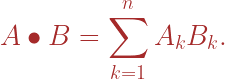
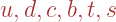
Einstein summation convention

Suppose you have a list of n numbers .

Their sum is often shorthanded using the Sigma notation like this

which is read “sum of from k=1 to k=n.” This letter k that varies from 1 to n is called an ‘index’.

Vectors. You can think of a vector as an ordered list of numbers

If you have two vectors  and their dot product is defined by multiplying their respective coordinates and adding the result:

Using our summation notation, we can abbreviate this to

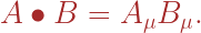
While working thru his general theory of relativity, Einstein noticed that whenever he was adding things like this, the same index k was repeated! (You can see the k appearing once in A and also in B.) So he thought, well in that case maybe we don’t need a Sigma notation! So remove it! The fact that we have a repeating index in a product expression would mean that a Sigma summation is implicitly understood. (Just don’t forget! And don’t eat fatty foods that can help you forget!)

With this idea, the Einstein summation convention would have us write the above dot product of vectors simply as

In his theory’s notation, it’s understood that the index k here would vary from 1 to 4, for the four dimensional space he was working with. That’s Einstein’s index notation where 1, 2, 3, are the indices for space coordinates (i.e., ), and k=4 for time (e.g., ). One could also write space-time coordinates using the vector where t is for time. 

(Some authors have k go from 0 to 3 instead, with k=0 corresponding to time and the others to space coordinates.)

I used ‘k’ because it’s not gonna scare anyone, but Einstein actually uses Greek letters like instead of the k. The convention is that Greek index letters range over all 4 space-time coordinates, and Latin indices (like k, j, m,etc)  for the space coordinates only. So if we use instead of k the dot product of the two vectors would be

So if we write it means we understand that we’re summing these over the 4 indices of space-time. And if we write  it means that we’re summing these over the 3 indices of space only. More specifically,

and

There is one thing that I left out of this because I didn’t want to complicate the introduction and thereby scare readers! (I already may have! Shucks!) And that is, when you take the dot product of two vectors in Relativity, their indices are supposed to be such that one index is a subscript (‘at the bottom’) and the other repeating index is a superscript (‘at the top’).  So instead of writing our dot product as it is written as

(This gets us into covariant vectors, ones written with subscripts, and contravariant vectors, ones written with superscripts. But that is another topic!)

How about we promote ourselves to Tensors? Fear not, let’s just treat it as a game with symbols! Well, tensors are just like vectors except that they can involved more than one index. For example, a vector such as in the above was written , so it involves one index . What if you have two indices? Well in that case we have a matrix which we can write . (Here, the two indices are sitting side by side like good friends and aren’t being multiplied! There’s an imaginary comma that’s supposed to separate them but it’s not conventional to insert a comma.)

The most important tensor in Relativity Theory is what is called the metric tensor written . It describes the distance structure (metric = distance) on a curved space-time. So much of the rest of the geometry of space, like its curvature, how to differentiate vector fields, curved motion of light and particles, shortest path in curved space between two points, etc, comes from this metric tensor .

The Einstein ‘gravitational tensor’ is one such tensor and is written . Tensors like those are called rank 2 tensors because they involve two different indices. Another good example of a rank 2 tensor is the energy-momentum tensor often written as . This tensor encodes the energy and matter distribution in spaces that dictate its geometry — the geometry (and curvature) being encoded in the Einstein tensor . (If you’ve read this far, you’re really getting into Relativity! And I’m very proud of you!)

You could have a tensors with 3, 4 or more indices, and the indices could be mixed subscripts and superscripts, like for example and .

If you have tensors like this, with more than 1 or 2 indices, you can still form their dot products. For example for the tensors D and F, you can take any lower index of D (say you take and set it equal to an upper index of F — and add! So we get a new tensor when we do this dot product! You get

where it is understood that since the index is repeated, you are summing over that index (from 1 to 4) (as I’ve written out on the right hand side). Notice that the indices that remain are . So this dot product gives rise to yet another tensor with these indices – let’s give the letter C:

.

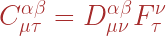
This process where you pick two indices from tensors and add their products along that index is called ‘contraction‘ – even though it came out of doing a simple idea of dot product. Notice that in general when you contract tensors the result is not a number but is in fact another tensor. This process of contraction is very important in relativity and geometry, yet it’s based on a simple idea, extended to complicated objects like tensors. (In fact, you can call the original dot product of two vectors a contraction too, except it would be number in this case.)

Thank you!

Einstein’s Religious Philosophy

Here is a short, sweet, and quick summary of some of Albert Einstein’s philosophy and religious views which I thought were interesting enough to jot down while I have that material fresh in mind. (I thought it’s good to read all these various views of Einstein’s in one fell swoop to get a good mental image of his views.) These can be found in most biographies on Einstein, but I included references [1] and [2] below for definiteness. (Throughout this note, ‘he’ refers, of course, to Einstein.) Let’s begin!

1. Einstein began to appreciate and identify more with his Jewish heritage in later life (as he approached 50).
2. He had profound faith in the order and discernible laws in the universe, which he said was the extent to which he calls himself ‘religious.’
3. God had no choice but to create the universe in the way He did.
4. He believed in something larger than himself, in a greater mind.
5. He called nationalism an infantile disease.
6. He received instruction in the Bible and Talmud. He is a Jew, but one who is also enthralled by “the luminous figure of the Nazarene.”
7. He believed Jesus was a real historical figure and that Jesus’ personality pulsates in every word in the Gospels.
8. He was not an atheist, but a kind of “deist.”
9. He did not like atheists quoting him in support of atheism.
10. He believed in an impersonal God, who is not concerned with human action.
11. His belief in an impersonal God was not disingenuous in order to cover up an underlying ‘atheism’.
12. He was neither theist nor atheist.
13. He did not believe in free will. He was a causal determinist. (Not even God has free will! 🙂 )
    
14. Though he did not believe in free will, nevertheless he said “I am compelled to act as if free will existed.”
15. He liked Baruch Spinoza’s treatment of the soul and body as one.
16. He did not believe in immortality.
17. He believed that the imagination was more important than knowledge.
18. He believed in a superior mind that reveals itself in world of experience, which he says represents his conception of God.
19. He believed in a “cosmic religious feeling” which he says “is the strongest and noblest motive for scientific research.”
20. “Science without religion is lame, religion without science is blind.”

There you have it, without commentary! 😉

References.

[1] Albert Einstein, Ideas and Opinions.

[2] Walter Isaacson, Einstein: His Life and Universe. (See especially chapter 17.)

======================================

Einstein and Pantheism

Albert Einstein’s views on religion and on the nature and existence of God has always generated interest, and they continue to. In this short note I point out that he expressed different views on whether he subscribed to “pantheism.” It is well-known that he said, for instance, that he does not believe in a personal God that one prays to, and that he rather believes in “Spinoza’s God” (in some “pantheistic” form). Here are two passages from Albert Einstein where he expressed contrary views on whether he is a “pantheist”.

“I’m not an atheist and I don’t think I can call myself a pantheist. We are in the position of a little child entering a huge library filled with books in many different languages.…The child dimly suspects a mysterious order in the arrangement of the books but doesn’t know what it is. That, it seems to me, is the attitude of even the most intelligent human being toward God.” (Quoted in Encyclopedia Britannica article on Einstein.)

Here, Einstein says that he does not think he can call himself a pantheist. However, in his book Ideas and Opinions he said that his conception of God may be described as “pantheistic” (in the sense of Spinoza’s):

“This firm belief, a belief bound up with a deep feeling, in a superior mind that reveals itself in the world of experience, represents my conception of God. In common parlance this may be described as “pantheistic” (Spinoza)” (Ideas and Opinions, section titled ‘On Scientific Truth’ – also quoted in Wikipedia with references)

It is true that Einsteins expressed his views on religion and God in various ways, but I thought that the fact that he appeared to identify and not identify with “pantheism” at various stages of his life is interesting. Setting aside that label, however, I think that his general conceptions of God in both these quotes — the mysterious order in the books, a universe already written in given languages, a superior mind that reveals itself in such ways — are fairly consistent, and also consistent with other sentiments he expressed elsewhere.

A game with Pi

Here’s an image of something I wrote down, took a photo of, and posted here for you. It’s a little game you can play with any irrational number. I took as an example.

You just learned about an important math concept/process called continued fraction expansions.

With it, you can get very precise rational number approximations for any irrational number to whatever degree of error tolerance you wish.

As an example, if you truncate the above last expansion where the 292 appears (so you omit the “1 over 292” part) you get the rational number 335/113 which approximates  to 6 decimal places. (Better than 22/7.)

You can do the same thing for other irrational numbers like the square root of 2 or 3. You get their own sequences of whole numbers.

Exercise: for the square root of 2, show that the sequence you get is
1, 2, 2, 2, 2, …
(all 2’s after the 1). For the square root of 3 the continued fraction sequence is
1, 1, 2, 1, 2, 1, 2, 1, 2, …
(so it starts with 1 and then the pair “1, 2” repeat periodically forever).

Matter and Antimatter don’t always annihilate

It is often said that when matter and antimatter come into contact they’ll annihilate each other, usually with the release of powerful energy (photons).

Though in essence true, the statement is not exactly correct (and so can be misleading).

For example, if a proton comes into contact with a positron they will not annihilate. (If you recall, the positron is the antiparticle of the electron.) But if a positron comes into contact with an electron then, yes, they will annihilate (yielding a photon). (Maybe they will not instantaneously annihilate, since they could for the minutest moment combine to form positronium, a particle they form as they dance together around their center of mass – and then they annihilate into a photon.)

The annihilation would occur between particles that are conjugate to each other — that is, they have to be of the same type but “opposite.” So you could have a whole bunch of protons come into contact with antimatter particles of other non-protons and there will not be mutual annihilation between the proton and these other antiparticles.

Another example. The meson particles are represented in the quark model by a quark-antiquark pair. Like this: . Here p and q could be any of the 6 known quarks and the  stands for the antiquark of . If we go by the loose logic that “matter and antimatter annihilate” then no mesons can exist since  and  will instantly destroy one another.

For example, the pion particle has quark content  consisting of an up-quark u and the anti-particle of the down quark. They don’t annihilate even though they’re together (in some mysterious fashion!) for a short while before it decays into other particles. For example, it is possible to have the decay reaction

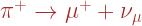
(which is not the same as annihilation into photons) of the pion into a muon and a neutrino.

Now if we consider quarkonium, i.e. a quark and its antiquark together, such as for instance or , so that you have a quark and its own antiquark, then they do annihilate. But, before they do so they’re together in a bound system giving life to the  particles for a very very short while (typically around seconds). They have a small chance to form a particle before they annihilate. It is indeed amazing to think how such Lilliputian time reactions are part of how the world is structured. Simply awesome! 😉

PS. The word “annihilate” usually has to do when photon energy particles are the result of the interaction, not simply as a result of when a particle decays into other particles.

Sources:

(1) Bruce Schumm, Deep Down Things. See Chapter 5, “Patterns in Nature,” of this wonderful book. 🙂

(2) David Griffiths, Introduction to Elementary Particles. See Chapter 2. This is an excellent textbook but much more advanced with lots of Mathematics!

Comparing huge numbers

Comparing huge numbers is often times not easy since you practically cannot write them out to compare their digits. (By ‘compare’ here we mean telling which number is greater (or smaller).) So it can sometimes be a challenge to determine.

Notation: recall that N! stands for  “N factorial,” which is defined to be the product of all positive whole numbers (starting with 1) up to and including N. (E.g., 5! = 120.) And as usual, Mⁿ stands for M raised to the power of n (sometimes also written as M^n).

Here are a couple examples of huge numbers (which we won’t bother writing out!) that aren’t so easy to compare but one of which is larger, just not clear which. I don’t have a technique except maybe in an ad hoc manner.

In each case, which of the following pairs of numbers is larger?

(1) (58!)² and 100!

(2) (281!)² and 500!

(3) (555!)² and 1000!

(4) 500!  and 10¹¹³⁴

(5) 399! + 400! and 401!

(6) 8²⁰⁰ and  9¹⁸⁹

(The last two of these are probably easiest.)

Have fun!

 

Escher Math

Escher Relativity

You’ve all seen these Escher drawings that seem to make sense locally but from a global, larger scale, do not – or ones that are just downright strange. We’ll it’s still creative art and it’s fun looking at them. They make you think in ways you probably didn’t. That’s Art!

Now I’ve been thinking if you can have similar things in math (or even physics). How about Escher math or Escher algebra?

Here’s a simple one I came up with, and see if you can ‘figure’ it out! 😉

(5 + {4 – 7)2 + 5}3.

LOL! 🙂

How about Escher Logic!? Wonder what that would be like. Is it associative / commutative? Escher proof?

Okay, so now … what’s your Escher?

Have a great day!

 

 

Richard Feynman on Erwin Schrödinger

I thought it is interesting to see what the great Nobel Laureate physicist Richard Feynman said about Erwin Schrödinger’s attempts to discover the famous Schrödinger equation in quantum mechanics (see quote below). It has been my experience in reading physics that this sort of “heuristic” reasoning is part of doing physics. It is a very creative (sometimes not logical!) art with mathematics in attempting to understand the physical world. Dirac did it too when he obtained his Dirac equation for the electron by pretending he could take the square root of the Klein-Gordon operator (which is second order in time). Creativity is a very big part of physics.

 

“When Schrödinger first wrote it down [his equation],

he gave a kind of derivation based on some heuristic

arguments and some brilliant intuitive guesses. Some

of the arguments he used were even false, but that does

not matter; the only important thing is that the ultimate

equation gives a correct description of nature.”

                                    — Richard P. Feynman

(Source: The Feynman Lectures on Physics, Vol. III, Chapter 16, 1965.)

 

 

 

How to see Schrödinger’s Cat as half-alive

Schrödinger’s Cat is a thought experiment used to illustrate the weirdness of quantum mechanics. Namely, unlike classical Newtonian mechanics where a particle can only be in one state at a given time, quantum theory says that it can be in two or more states ‘at the same time’. The latter is often referred to as ‘superposition’ of states.

If D refers to the state that the cat is dead, and if A is the state that the cat is alive, then classically we can only have either A or D at any given time — we cannot have both states or neither.

In quantum theory, however, we can not only have states A and D but can also have many more states, such a for example this combination or superposition state:

ψ = 0.8A + 0.6D.

Notice that the coefficient numbers 0.8 and 0.6 here have their squares adding up to exactly 1:

(0.8)² + (0.6)² = 0.64 + 0.36 = 1.

This is because these squares, (0.8)² and (0.6)², refer to the probabilities associated to states A and D, respectively. Interpretation: there is a 64% chance that this mixed state ψ will collapse to the state A (cat is alive) and a 36% chance it will collapse to D (cat is dead) — if one proceeds to measure or find out the status of the cat were it to be in a quantum mechanical state described by ψ.

Realistically, it is hard to comprehend that a cat can be described by such a state. Well, maybe it isn’t that hard if we had some information about the probability of decay of the radioactive substance inside the box.

Nevertheless, I thought to share another related experiment where one could better ‘see’ and appreciate superposition states like ψ above. The great physicist Richard Feynman did a great job illustrating this with his use of the Stern-Gerlach experiment (which I will tell you about). (See chapters 5 and 6 of Volume III of the Feynman Lectures on Physics.)

In this experiment we have a magnetic field with north/south poles as shown. Then you have a beam of spin-half particles coming out of a furnace heading toward the magnetic field. The result is that the beam of particles will split into two beams. What essentially happened is that the magnetic field made a ‘measurement’ of the spins and some of them turned into spin-up particles (the upper half of the split beam) and the others into spin-down (the bottom beam). So the incoming beam from the furnace is like the cat being in the superposition state ψ and magnetic field is the agent that determined — measured! — whether the cat is alive (upper beam) or dead (lower beam). (Often in physics books they use the Dirac notation |↑〉for spin-up state and |↓〉 for spin-down.)

In a way, you can now see the initial beam emanating from the furnace as being in a superposition state.

Ok, so the superposition state of the initial beam has now collapsed the state of each particle into two specific states: spin-up state (upper beam) and the spin-down state (lower beam). Does this mean that these states are no longer superposition states?

Yes and No! They are no longer in superposition if the split beams enter another magnetic field that points in the same direction as the original one. If you pass the upper beam into a second identical magnetic field, it will remain an upper beam — and the same with the lower beam. The magnetic field ‘made a decision’ and it’s going to stick with it! 🙂

That is why we call these states (upper and lower beams) ‘eigenstates’ of the original magnetic field. They are no longer mixed superposition states — the cat is either dead or alive as far as this field is concerned and not in any ‘in between fuzzy’ states.

Ok, that addresses the “Yes” part of the answer. Now for the “No” part.

Let’s suppose we have a different magnetic field, one just like the original one but perpendicular in direction to it. (So it’s like you’ve rotated the original field by 90 degrees; you can rotate by a different angle as well.)

In this case if you pass the original upper beam (that was split by the first magnetic field) into the second perpendicular field, this upper beam will split into two beams! So with respect to the second field the upper beam is now in a superposition state!

Essential Principle: the notion of superposition (in quantum theory) is always with respect to a variable that is being measured. In our case, that variable is the magnetic field. (And here we have two magnetic fields, hence we have two different variables — non-commuting variables as we say in quantum theory.)

Therefore, what was an eigenstate (collapsed state) for the first field (the upper beam) is no longer an eigenstate (no longer ‘collapsed’) for the second (perpendicular) field. (So if a wavefunction is collapsed, it can collapse again and again!)

The Schrodinger Cat experiment could possibly be better understood not as one single experiment, but as a stream of many many boxes with cats in them. This view might better relate to the fact that we have beam of particles each of which is being ‘measured’ by the field to determine its spin status (as being up or down).

Best wishes, Sam

Reference. R. Feynman, R. Leighton, M. Sands, The Feynman Lectures on Physics, Vol. III (Quantum Mechanics), chapters 5 and 6.

Postscript. It occurred to me to add a uniquely quantum mechanical feature that is contrary to classical physics thinking.   The Stern-Gerlach experiment is a good place to see this feature.

We noted that when the spin-half particles emerge from the furnace and into the magnetic field, they split into upper and lower beams. Classically, one might think that before entering the field the particles already had their spins either up or down before a measurement takes place (i.e., before entering the magnetic field) — just as one might say that the earth has a certain velocity as it moves around the sun before we measure it. Quantum theory does not see it that way. In the predominant Copenhagen Interpretation of quantum theory, one cannot say that the particle spins were already a mix of up or down spins before entering the field. Reason we cannot say this is that if we had rotated the field at an angle (say at right angles to the original), the beams would still split into two, but not the same two beams as before! So we cannot say that the particles were already in a mix of those that had spins in one direction or the other. That is one of the strange features of quantum theory, but wonderfully illustrated by Stern-Gerlack.

Mathematics. In vector space theory there is a neat way to illustrate this quantum phenomenon by means of `bases’. For example, the vectors (1,0) and (0,1) form a basis for 2D Euclidean space R². So any vector (x,y) can be expressed (uniquely!) as a superposition of them; thus,

(x,y) = x(1,0) + y(0,1).

So this would be, to make an analogy, like how the beam of particles, described by (x,y), can be split into to beams — described by the basis vectors (1,0) and (0,1).

However, there are a myriad of other bases. For example, (2,1) and (1,1) also form a basis for R². A general vector (x,y) can still be expressed in terms of a superposition of these two:

(x,y) = a(2,1) + b(1,1)

for some constants a and b (which are easy to solve in terms of x, y). So this other basis could, by analogy, represent a magnetic field that is at an angle with respect to the original — and its associated beams (2,1) and (1,1) (it’s eigenstates!) would be different because of their different directions. As a matter of fact, we can see here that these eigenstates (collapsed states), represented by (2,1) and (1,1), are actual (uncollapsed) superpositions of the former two, namely (1,0) and (0,1). And vice versa!

Analogy: let’s suppose the vector (5,3) represents the particle states coming out of the furnace. Let’s think of the basis vectors (1,0) and (0,1) represent the spin-up and spin-down beams, respectively, as they enter the first magnetic field, and let the other basis vectors (2,1) and (1,1) represent the spin-up and spin-down beams when they enter the second rotated (maybe perpendicular) magnetic field. Then the particle state (5,3) is a superposition in each of these bases!

(5,3) = 5(1,0) + 3(0,1),

(5,3) = 2(2,1) + 1(1,1).

So it is now quite conceivable that the initial mixed state of particles as they exit the furnace can in fact split in any number of ways as they enter any magnetic field! I.e., it’s not as though they were initially all either (1,0),(0,1) or (2,1),(1,1), but (5,3) could be a simultaneous combination of each — and in fact (5,3) can be combination (superposition) in an infinite number of bases.

Indeed, it now looks like this strange feature of quantum theory can be described naturally from a mathematical perspective! Vector Space bases furnish a great example!

**********************************************************

Principles of quantum theory

One beautiful summer morning I spent a couple hours in a park reflecting on what I know about quantum mechanics and thought to sketch it out from memory. (A good brain exercise to recapture things you learned and admire.) This note is an edited summary of my handwritten draft (without too much math).

Being a big subject, I will stick to some basic ideas (or principles) of quantum theory that may be worth noting.

Two key concepts are that of a `state’ and that of an ‘observable’.

The former describes the state of the system under study. The observable is a thing we measure. So for example, an electron can be in the ground state of an atom – which means that it is in `orbital’ of lowest energy. Then we have other states that it can be in at higher energies.

The observable is a quantity distinct from a state and one that we measure. Such as for example measuring a particle’s energy, its mass, position, momentum, velocity, charge, spin, angular momentum, etc.

QM gives us principles / interpretations by how states and observables can be mathematically described and how they relate to one another. So here is the first principle.

Principle 1. The state of a system is described by a function (or vector) ψ. The probability density associated with it is given by |ψ|².

This vector is usually a mathematical function of space, time (sometime momentum) variables.

For example, f(x) = exp(-x^2) is one such example. You can also have wave examples such as g(x) = exp(-x^2) sin(x) which looks like a localized wave (a packet) that captures both being a particle (localized) and a wave (due to the wave nature of sin(x)). This wave nature of the function allows it to interfere constructively or destructively with other similar functions — so you can have interference! In actual QM these wavefunctions involve more variables that one x variable, but I used one variable to illustrate.

Principle 2. Each measurable quantity (called an ‘observable’) in an experiment is represented by a matrix A. (A Hermitian matrix or operator.)

For example, energy is represented by the Hamiltonian matrix H, which gives the energy of a system under study. The system could be the hydrogen atom. In many or most situations, the Hamiltonian is the sum of the kinetic energy plus the potential energy (H = K.E. + V).

For simplicity, I will treat a measurable quantity and its associated matrix on equal footing.

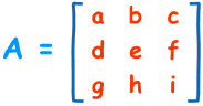
From matrix algebra, a matrix is a rectangular array of numbers – like, say, a square array of 3 by 3 numbers, like this one I grabbed from the net:

Turns out you can multiply such things and do some algebra with them.

Two basic facts about these matrices is:

(1) they generally do not have the commutative property (so AB and BA aren’t always equal), unlike real or complex numbers,

(2) each matrix A comes with `magic’ numbers associated to it called eigenvalues of A.

For example the matrix

(called diagonal because it has all zeros above and below the diagonal) has eigenvalues 1, 4, -3. (When a matrix is not diagonal we have a procedure for finding them. Study Matrix or Linear Algebra!)

Principle 3. The possible measurements of a quantity will be its eigenvalues.

For example, the possible energy levels of an electron in the hydrogen atom are eigenvalues of the associated Hamiltonian matrix!

Principle 4. When you measure a quantity A when the system is in the state ψ the system `collapses’ into an eigenstate f of the matrix A.

Therefore the system makes a transition from state ψ to state f (when A is measured).

So mathematically we write

Af = af

which means that f is an eignstate (or eigenvector) of A with eigenvalue a.

So if A represents energy then `a’ would be energy measurement when the system is in state f.

For a general state ψ we cannot say that Aψ = aψ. This eigenvalue equation is only true for eigenstates, not general states.

Principle 5. Each state ψ of the system can be expressed as a superposition sum of the eigenstates of the measurable quantity (or matrix) A.

So if f, g, h, … are the eigenstates of A, then any other state ψ of the system can be expressed as a superposition (or linear combination) of them:

ψ = bf + cg + dh + …

where b, c, d, … are (complex) numbers. Further, |c|^2 = probability ψ will `collapse’ into the eigenstate g when measurement of A is performed.

These principles illustrate the indeterministic nature of quantum theory, because when measurement of A is made, the system can collapse into any one of its many eigenstates (of the matrix A) with various probabilities. So even if you had the ‘exact same’ setup initially there is no guarantee that you would see your system state change into the same state each time. That’s non-causality! (Quite unlike Newtonian mechanics.)

Principle 6. (Follow-up to Principles 4 and 5.) When measurement of A in the state ψ is performed, the probability that the system will collapse into the eigenstate vector φ is the dot product of Aψ and φ.

The latter dot product is usually written using the Dirac notation as <φ|A|ψ>.  In the notation above, this would be same as |c|^2.

Next to the basic eigenvalues of A, there’s also it’s `average’ value or expectation value in a given state. That’s like taking the weighted average of tests in a class – with weights assigned to each eigenstate based on the superposition (as in the weights b, c, d, … in the above superposition for ψ). So we have:

Principle 7. The expected or average value of quantity A in the state described by ψ is <ψ|A|ψ>.

In our notation above where ψ = bf + cg + dh + …, this expected value is

<ψ|A|ψ> = |b|^2 times (eigenvalue of f)  + |c|^2 times (eigenvalue of g) + …

which you can see it being the weighed average of the possible outcomes of A, namely from the eigenvalues, each being weighted according to its corresponding probabilities |b|^2, |c|^2, … .

In other words if you carry out measurements of A many many times and calculate the average of the values you get, you get this value.

Principle 8. There are some key complementary measurement observables. (Classic example: Heisenberg relation QP – PQ = ih.)

This means that if you have two quantities P and Q that you could measure, if you measure P first and then Q, you will not get the same result as when you do Q first and then P. (In Newton’s mechanics, you could at least in theory measure P and Q simultaneously to any precision in any order.)

Example, position and momentum are complementary in this respect — which is what leads to the Heisenberg Uncertainty Principle, that you cannot measure both the position and momentum of a subatomic particle with arbitrary precision. I.e., there will be an inherent uncertainty in the measurements. Trying to be very accurate with one means you lose accuracy with they other all the more.

From Principle 8 you can show that if you have an eigenstate of the position observable Q, it will not be an eigenstate for P but will be a superposition for P.

So `collapsed’ states could still be superpositions! (Specifically, a collapsed state for Q will be a superposition, uncollapsed, state for P.)

That’s enough for now. There are of course other principles (and some of the above are interlinked), like the Schrodinger equation or the Dirac equation, which tell us what law the state ψ must obey, but I shall leave them out. The above should give an idea of the fundamental principles on which the theory is based.

Have fun,
Samuel Prime

The 21 cm line of hydrogen in Radio Astronomy

 

This has been a wonderful discovery back in the 1950s that gave Radio Astronomy a good push forward. It also helped in mapping out our Milky Way galaxy (which we really can’t see very well!).

It arose from a feature of quantum field theory, specifically from the hyperfine structure of hydrogen. (I’ll try to explain.)

You know that the hydrogen atom consists of a single proton at its central nucleus and a single electron moving around it somehow in certain specific quantized orbits. It cannot just circle around in any orbit.

That was one of Niels Bohr’s major contributions to our understanding of the atom. In fact this year we’re celebrating the 100th anniversary of his model of the atom (his major papers written in 1913). Some articles in the June issue of Nature magazine are in honor of Bohr’s work.

Normally the electron circles in the lowest orbit associated with the lowest energy state – usually called the ground state (the one with n = 1).

It is known that protons and electrons are particles that have “spin”. (That’s why they are sometimes also called ‘fermions’.) It’s as if they behave like spinning tops. (The Earth and Milky Way are spinning too!)

The spin can be in one direction (say ‘up’) or in the other direction (we label as ‘down’). (These labels of where ‘up’ and ‘down’ are depends on the coordinates we choose, but let’s now worry about that.)

When scientists looked at the spectrum of hydrogen more closely they saw that even while the electron can be in the same ground state – and with definite smallest energy – it can have slightly different energies that are very very close to one another. That’s what is meant by “hyperfine structure” — meaning that the usual energy levels of hydrogen are basically correct except that there are ever so slight deviations from the normal energy levels.

It was discovered by means of quantum field theory that this difference in ground state energies arise when the electron and proton switch between spinning in the same direction to spinning in opposite directions (or vice versa).

When they spin in the same direction the hydrogen atom has slightly more energy than when they are spinning in opposite direction.

And the difference between them?

The difference in these energies corresponds to an electromagnetic wave corresponding to about 21 cm wavelength. And that falls in the radio band of the electromagnetic spectrum.

So when the hydrogen atom shows an emission or absorption spectrum in that wavelength level it means that the electron and proton have switched between having parallel spins to having opposite spins. When the switch happens you see an electromagnetic ray either emitted or absorbed.

It does not happen too often, but when you have a huge number of hydrogen atoms — as you would in hydrogen clouds in our galaxy — it will invariably happen and can be measured.

Now it’s a really nice thing that our galaxy contains several hydrogen clouds.  So by measuring the Doppler shift in the spectrum of hydrogen — at the 21 cm line! — you can measure the velocities of these clouds in relation to our location near the sun.

These velocity distributions are used together with other techniques to map out the hydrogen clouds in order to map out and locate the spiral arms they fall into.

That work (lots of hard work!) showed astronomers that our Milky Way does indeed have arms, just as we would see in some other galaxies, such as in the picture shown here of NGC 1232.

The one UNKNOWN about the structure of our Milky Way is that we don’t know whether it has 2 or 4 arms.

References:
[1] University Astronomy, by Pasachoff and Kutner. 
[2] Astronomy (The Evolving Universe), by Michael Zeilik.

(These are excellent sources, by the way.)

August Kekule’s Benzene Vision

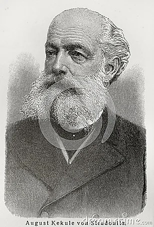
The first time I heard of August Kekule’s dream/vision was from my dear mother! (My mom is a geologist who obviously had to know a lot of chemistry.)  I am referring to Kekule’s vision while gazing at a fireplace which somehow prompted him onto the idea for the structure of the benzene molecule C₆H₆. And then I heard that the story is suspect maybe even a myth cooked up by unscientific minds. Now I have learned that Kekule himself recounted that story which was translated into English and published in the Journal of Chemical Education (Volume 35, No. 1, Jan. 1958, pp 21-23, translator: Theodor Benfey). Here is an excerpt from that paper relevant to the story where Kekule talks about his discovery.

I was sitting writing at my textbook but the work did not progress; my thoughts were elsewhere. I turned my chair to the fire and dozed. Again the atoms were gamboling before my eyes. This time the smaller groups kept modestly in the background.    My mental eye, rendered more acute by repeated visions of the kind, could now distinguish larger structures of manifold conformation: long rows, sometimes more closely fitted together all twining and twisting in snake-like motion. But look! What was that? One of the snakes had seized hold of its own tail, and the form whirled mockingly before my eyes.    As if by a flash of lightning I awoke; and this time also I spent the rest of the night in working out the consequences of the hypothesis. Let us learn to dream, gentlemen, then perhaps we shall find the truth.

And to those who don’t think The truth will be given. They’ll have it without effort.

But let us beware of publishing our dreams till they have been tested by the making understanding.

Countless spores of the inner life fill the universe, but only in a few rare beings do they find the soil for their development; in them the idea, whose origin is known to no men, comes to life in creative action.  (J. Von Liebig)

I believe it is unnecessary to rule out or ridicule dreams, trances, visions in the pursuit of scientific truth. Because, after all, they still have to be tested and examined in our sober existence (as Kekule already alluded). I see them as extensions of thinking and contemplation, and surely there is nothing wrong with these.

Einstein on theory, logic, reality

 

Long ago (late 1980s) I attended a lecture by Einstein biographer I. Bernard Cohen. (Cohen actually interviewed Einstein and published it in the Scientific American in the 1955 issue.)

 
In his lecture, Cohen described Einstein’s view of scientific discovery as a sort of ‘leap’ from experiences to theory. That theory is not logically deduced from experiences but that theory is “jumped at” — or “swooped” is the word Cohen used, I think — thru the imagination or intuition based on our experiences (which of course would/could include experiments). This reminds one of the known Einstein quote that “imagination is more important that knowledge.”

In his book Ideas and Opinions, Albert Einstein said:

“Pure logical thinking cannot yield us any knowledge of the empirical world; all knowledge of reality starts from experience and end in it. Propositions arrived at by purely logical means are completely empty as regards reality. Because Galileo saw this, and particularly because he drummed it into the scientific world, he is the father of modern physics—indeed, of modern science altogether.”

(See Part V of his “Ideas and Opinions” in the section entitled “On the Method of Theoretical Physics.”)

In a related passage from the same section, Einstein noted:

“If, then, it is true that the axiomatic foundation of theoretical physics cannot be extracted from experience but must be freely invented, may we ever hope to find the right way? Furthermore, does this right way exist anywhere other than in our illusions? May we hope to be guided safely by experience at all, if there exist theories (such as classical mechanics) which to a large extent do justice to experience, without comprehending the matter in a deep way?

To these questions, I answer with complete confidence, that, in my opinion, the right way exists, and that we are capable of finding it. Our experience hitherto justifies us in trusting that nature is the realization of the simplest that is mathematically conceivable. I am convinced that purely mathematical construction enables us to find those concepts and those lawlike connections between them that provide the key to the understanding of natural phenomena. Useful mathematical concepts may well be suggested by experience, but in no way can they be derived from it. Experience naturally remains the sole criterion of the usefulness of a mathematical construction for physics. But the actual creative principle lies in mathematics. Thus, in a certain sense, I take it to be true that pure thought can grasp the real, as the ancients had dreamed.”

Note his reference to theory as being ‘freely invented’ (and even ‘illusion’) which echo the role of intuition and imagination in the scientific development of theory (but which are probably not completely divorced from experience either!).

The last two quotes above incidentally can be found online in Standford’s Encyclopedia of Philosophy: Einstein’s Philosophy of Science

 

The sphere in dimensions 4, 5, …

The volume of a sphere of radius R in 2 dimensions is just the area of a circle which is π R². (The symbol π is Pi which is 3.1415….)

The volume of a sphere of radius R in 3 dimensions is (4/3) π R³.

The volume of a sphere of radius R in 4 dimensions is (1/2) π² R⁴.

Hold everything! How’d you get that? With a little calculus!

Ok, you see a sort of pattern here. The volume of a sphere in n dimensions has a nice form: it is some constant C(n) (involving π and some fractions) times the radius R raised to the dimension n:

V(n,R) = C(n) Rⁿ —————– (1)

where I wrote V(n,R) for the volume of a sphere in n dimensions of radius R (as a function of these two variables).

Now, how do you get the constants C(n)?

With a bit of calculus and some ‘telescoping’ as we say in Math.

(In the cases n = 2 and n = 3, we can see that C(2) = π, and C(3) = 4π/3.)

First, let’s do the calculus. The volume of a sphere in n dimensions can be obtained by integrating the volume of a sphere in n-1 dimensions like this using the form (1):

V(n,R) = ∫ V(n-1,r) dz = ∫ C(n-1) r^n-1 dz

where here r² + z² = R² and your integral goes from -R to R (or you can take 2 times the integral from 0 to R). You solve the latter for r, plug it into the last integral, and compute it using the trig substitution z = R sin θ. When you do, you get

V(n,R) = 2C(n-1) Rⁿ ∫ cosⁿθ dθ.

The cosine integral here goes from 0 to π/2, and it can be expressed in terms of the Gamma function Γ, so it becomes

V(n,R) = 2C(n-1) Rⁿ π^1/2 Γ((n+1)/2) / Γ((n+2)/2).

Now compare this with the form for V in equation (1), you see that the R’s cancel and you have C(n) expressed in terms of C(n-1). After telescoping and simplifying you eventually get the volume of a sphere in n dimensions to be:

V(n,R) = π^n/2 Rⁿ / Γ((n+2)/2).

Now plug in n equals 4 dimensions and you have what we said above. (Note: Γ(3) = 2 — in fact, for positive integers N the Gamma function has simple values given by Γ(N) = (N-1)!, using the factorial notation.)

How about the volume of a sphere in 5 dimensions?  It works out to

V(5,R) = (8/15) π² R⁵.

One last thing that’s neat: if you take the derivative of the Volume with respect to the radius R, you get its Surface Area!  How crazy is that?!!

Can a product of 4 consecutive odds be a perfect square?

Someone on twitter asked if a product of four consecutive odd positive numbers can be a perfect square.

My answer: No.

For example, 3 x 5 x 7 x 9 = 945 which is not a perfect square. (30^2 = 900 and 31^2 = 961.) Similarly, 7 x 9 x 11 x 13 = 9009, again is not a perfect square.

Here is my proof. Write the four consecutive positive odd numbers as:

2x+1, 2x+3, 2x+5, 2x+7

where x is a positive integer.

The middle two numbers 2x+3, 2x+5 cannot both be perfect squares since their difference is 2 — the difference between two positive consecutive perfect squares is at least 3. Let’s suppose it is 2x+3 that is not a perfect square. (The argument can still be adapted if it was 2x+5.) So 2x+3 is divisible by an odd prime p that has an odd power in its prime factorization. This prime p cannot divide the other three factors 2x+1, 2x+5, 2x+7, or else it would divide their differences from 2x+3, which are 2 or 4 (and p is odd). Therefore the prime p appears in the prime factorization of the product

(2x+1)(2x+3)(2x+5)(2x+7)

with only an odd power, hence this product cannot be a perfect square. QED

Progress on the Twin Prime Conjecture

The Chinese mathematician Yitang Zhang made great strides in one of the big problems in number theory called the Twin Prime Conjecture. He did not solve it but proved a related result that is considered quite remarkable — and he got his paper accepted for publication in the very prestigious math journal Annals of Mathematics.

If you wish you can read the sources below regarding the news on this, but I’d like to say things my way.

First, let’s explain some things. The ‘numbers‘ we’re talking about here are mainly positive whole numbers 1, 2, 3, 4, …, (which we call positive integers, or natural numbers). (So we’re not talking fractions here.)

A number is prime when it is not divisible by any other number beside 1 and itself. So for example, 5 is a prime, while 6 is not prime (we call it composite, since it is divisible by 2 and 3, beside 1 and 6).

So the sequence of prime numbers starts off and proceeds like this:

2, 3, 5, 7, 11, 13, 17, 19, 23, 29, 31, 37, 41, 43, 47, 53, 59, 61, 67, 71, 73, 79, 83, 89, 97, 101, …

and they go on and on forever. We know that there are infinitely many prime numbers (and the proof is not hard).

Now if you look closely at this list of primes, you notice something interesting. That there are ‘consecutive’ pairs of primes. Ones whose difference is 2.  Like the pair 5, 7, and the pair 11, 13, and the pair 29, 31, etc etc. These are called twin primes.

The Twin Prime Conjecture says that there are infinitely many of these twin pairs of primes.

But unlike Euclid’s proof that there are infinitely many primes (which is easy), the proof of the Twin Prime conjecture is extremely hard or just unknown. (Or maybe it’s not true!) No one has been able (so far) to settle the question or find a proof of it.

Since that is too hard, mathematicians try to ask and maybe settle simpler, but related, questions that they may have a chance at answering.

For example, instead of looking at pairs of primes whose difference is 2, why not look at ones whose difference is some number L?

As a related conjecture, one can ask:

Q: Is there a number L such that there are infinitely many pairs of primes whose difference is no more than L?

When L = 2, this question reduces to the Twin Prime Conjecture. For L = 10, let’s say, we can have pairs like 7, 11, whose difference is 4 which is no more than 10. Another pair would be 17, 23, whose difference is 6 (again no more than 10). Etc.

Now what Professor Yitang Zhang proved is that the answer to question Q is YES! There is such a fixed difference L. He proved that if you take L to be 70,000,000 (70 million) then there are infinitely many pairs of primes whose difference is no more than 70 million.

(So in particular we don’t know if there infinitely many pairs of primes whose difference is not more than 100 (or 1000, or even a million). These would still be interesting but apparently quite hard to answer.)

Once again, we have very simple sounding questions (a babe can ask them!) that are very hard to prove, and indeed we do not even have proofs for them.

REFERENCES:

These two reference are short reports on the result.

Nature Magazine — New Scientist

The following reference is slightly longer and more detailed:

Simon’s Foundation

Brzezinski on US policy on Iran

Zbigniew Brzezinski wrote an op-ed article in the Washington Post, titled “Iran should be key topic at hearings,” in which he basically said that the US should just continue to stick with a policy of sanctions and more sanction, until (maybe, hopefully) Iran caves in.

Brzezinski’s policy on Iran, however, is that of containment.  Obama himself specifically said that containment is not his policy.

Secondly, the outcome of Brzezinski’s policy is that it is ok for Iran to gain influence and even acquire nukes in order to destabilize the region and our alies therein.

Thirdly, his position does not address the dangerous and real possibility that economic sanctions on Iran will have little or no effect in stopping Iran’s ability and objective to acquire nuclear weapons.  From what we’ve seen so far, and in view of the IAEA reports that have been coming out during the last year or two, Iran’s nuclear program has been progressing and progressing in spite of severe sanctions. (Brzezinski never addressed this point.) So the sanctions are hurting Iran but there are many loopholes that Iran can and has exploited.

Fourthly, the doomsday scenarios he’s cooking up hardly happened even with US invasion of Iraq and Afghanistan.  Plus, he conveniently ignores doomsday scenarios resulting from his policy. (How about Iran’s inciting genocide against Israel as a doomsday scenario?) He never cared about that.

In sum, his position is untenable and is just the kind of policy that further endangers the region, our allies and our interests. It is a policy that promotes and aids the proliferation of dangerous rogue regimes like Iran.